BAYES FILTER
To be successful, a robotic system (hereinafter also referred to as a “robot”) must be capable of dealing suitably the enormous uncertainty that exists in the physical world, which is due to a number of factors: highly dynamic and unpredictable environment, sensors limited in range and resolution, as well as subject to noise and faults, not completely predictable and reliable actuators, especially in low-cost systems, software that is based on approximate models and algorithms (often minor quantities that influence the phenomenon cannot be taken into account).
So, the state of the robotic system cannot be determined exactly, but must be estimated evaluating uncertainty. Uncertainty can be explicitly represented using the calculation of probabilities. The problems that can be treated with this methodology are:
a) perception (through sensors);
b) planning and control (through actuators).
Basically, probabilistic models are more robust with regard to the problems set out above; this allows them to scale better in complex real environments. They can also work well even if they are not very accurate. However, probabilistic models introduce greater computational complexity than their deterministic counterparts, due to the fact that they must deal with probability density functions rather than single values; for this reason, the corresponding algorithms must be approximated. This problem was mitigated in recent times by the increase in the computational capacity of processors.
State estimation
The central problem is the estimation of the state, starting from the data provided by sensors, that is, from the measurements. The state cannot be observed directly but must be inferred, in a probabilistic way, on the basis of all past actions and all past measurements, creating the so-called "beliefs" (the supposed states). Furthermore, the same measurements are corrupted by noise / sensor limits and therefore their true values must also be estimated. Even the effects of the actions that can be carried out by the robot cannot be determined a priori with absolute accuracy. It is generally assumed that the stochastic variables representing each future state 𝑥𝑡 + 𝑛 are dependent only from the state at instant 𝑥𝑡 and not from the previous 𝑥𝑡 − 𝑛 (assumption of the Markovian chain). The Markovian hypothesis is valid only if the state includes all possible phenomena relevant to the behavior of the robot, if the probabilistic models are accurate enough, if the probability functions are accurate enough and if each control variable of the robot affects a single control.
This situation is also made complex by the existence of hidden variables (and therefore easily overlooked by the designer) that influence the state; the more these variables are important, the more the output of the model that does not consider them tends to be totally random (and therefore useless) producing flat probability distributions. On the contrary, if these variables have a minor effect compared to those explicitly considered, their contribution can be implicitly represented by the whole probabilistic modeling of the sensor measurement process (a very trivial example is the effect of temperature, which in certain processes can be substantial both qualitatively and quantitatively, being negligible in other ones and so implicitly representable by proper probability distribution of the other variables).
It is also important to properly estimate the correlations that exist between the variables that regulate the process: neglecting the weak dependencies between them permits to avoid the combinatorial explosion, so to reduce time-complexity of the algorithm.
As previously mentioned, the operation of a robotic system consists of a measurement process named "observation" and of a control process named "action" during which the robot operates the actuators. Measuring tends to increase the level of information about the state, while the control action tends to decrease this level. Both of these phases contribute to the estimation of the state (i.e. to the determination of beliefs).
Discrete Bayes filter
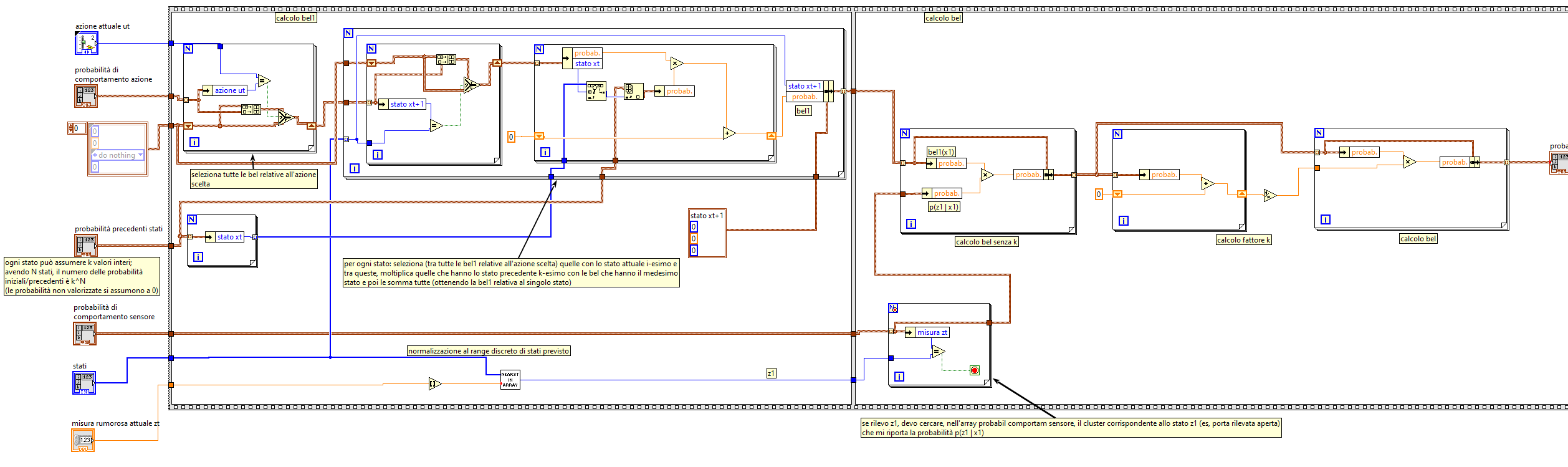
It can be used when the number of states is finite (discrete state variables, that is, they can assume a finite set of values). It is a recursive algorithm that computes bel (beliefs, the supposed states) (𝑥𝑡 ) starting from measurements 𝑧𝑡 and control data 𝑢𝑡 . Every execution (calling) of the Bayes_filter function is related to a single instant in time; within the function itself, the for loop iterates for each possible value of the status variable:
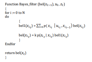
Bayes filter
where "bel1" is the control update and "bel" is the measurement update.
The probability of the current state (actual measure) is determined from:
1) measurement (noisy);
2) probabilities of sensor behavior (a-priori);
3) probability of action behavior (a-priori);
4) previous probabilities of the state (from previous Bayes filter calculations);
5) action performed.
In summary, if sensors become unreliable in some instants (giving noisy or unreliable measurements), the measurements themselves (which indicate system status) are corrected based on the previous experience about sensors and system behavior related to the action and based on the previous status probabilities.